.jpg)
Investigating the Linear Relationship between GDP and CO2 Emissions Globally
- Aisha Syed
- Oct 11, 2022
- 6 min read

The following report was a final project for CEE 202: Engineering Risk and Uncertainty.
Authors: Riley Kelch, Hongjie Luo, Emily Shao, Aisha Syed, and Alan Wagner
Date Submitted: 09 December 2021
Abstract
This paper investigates the linear relationship between GDP and CO2 emissions globally using simple linear regression. CO2 emissions is an important topic, as climate change becomes a developing global issue which impacts the natural environment, and identifying a relationship with GDP allows us to draw conclusions about economic activity and climate change. We found that though β1=2.63(p<0.05), the assumptions of a linear regression model are not completely met when influential points are eliminated from the data. It was concluded that further work needs to be done in order to determine if there is a linear relationship between the two variables.
Introduction
This paper will investigate if there is a linear relationship between GDP and CO2 emissions globally in 2018. As climate change continues to be a contentious topic, the analysis of carbon emission patterns is essential in determining the magnitude of the situation. This can be accomplished by identifying where carbon emissions levels need to be lowered the most and implementing proper solutions to the issue.
Since the ramifications of carbon in the atmosphere affect not only the human population, but the ecosystem as a whole (Taub, 2010), it is urgent that action be taken to reduce and regulate the impacts of climate change. An important consideration in this analysis includes the relationship between CO2 emissions and GDP, as “GDP is the most commonly used measure of economic activity” (FocusEconomics, 2014), and industry is one of the largest sources of CO₂ production. According to the International Energy Agency: China, America, India are the three countries that emit the highest levels of carbon dioxide emission, while Saudi Arabia, Kazakhstan, and Australia are the countries with the highest levels of carbon dioxide per capita.
Important descriptive statistics for the variables of CO2 emissions and GDP is as follows: The mean for CO2 emissions is 179.53 megatons and 454.13 billion USD for GDP. The standard deviation is 867.67 megatons for CO₂ and 1908.08 billion USD for GDP.
Data and Methods
Due to the previously stated analysis considerations, the variables we are considering are CO₂ emissions (in megatons), and GDP (billion US dollars) in 2018 for all countries with available data. Data concerning these variables can be found in the World Bank DataBank. This data is meant to represent a comparison between each country’s respective CO₂ emissions and GDP, allowing for a conclusion to be drawn as to whether or not the two sets of data have a linear relationship. 13 of the most influential points were removed from the data before analysis.
The null hypothesis is that there is no linear relationship between GDP and CO2 Emissions, or H0=β1=0, and the alternative hypothesis is that there is a linear relationship between the two variables, or H1=β10.
When creating a simple linear regression model, the following assumptions are made: GDP is independent, GDP can be described by a linear function of CO2 emissions, variations of observations around the regression line is constant, and residuals are normally distributed. To check the validity of this assumption, relations of the two variables will be found and diagnostic plots will be evaluated. A correlation coefficient r that has an absolute value close to 1 indicates that there is a strong correlation. A positive value indicates a positive correlation while a negative value indicates a negative correlation.
Results and Discussion
In order to determine whether or not the GDP per country has a direct impact on CO₂ emission, we must reject the null hypothesis, which states that there is no linear relationship between GDP and CO₂ emissions, or that the slope β1=0. Using linear regression at a level of significance of 0.05, we are evaluating if there is a linear relationship between GDP and CO2 emissions by checking if the assumptions of linear regressions are met and if β1=0.

Figure 1. Scatterplot
Figure 1 shows a scatterplot of GDP vs CO2 emissions with the red line indicating the linear regression line. Plotting GDP directly against CO2 emissions in a scatterplot graph displays the relationship between the two variables. The trend line indicates a positive linear relationship between GDP and CO2 emissions as both variables increase with respect to one another. While this makes a strong case to reject the null hypothesis, we cannot actually confirm a linear relationship between the two variables based off of the scatterplot alone.

Figure 2. Linear model summary
As shown in Figure 2, the best fit equation that relates GDP to CO2 emissions is GDP(billion USD) = 2.63*CO2Emissions(Mt) + 41.The slope of the best fit line is β1=2.630 and is statistically significant, as p<2e-16 and therefore p<0.05. The intercept is not statistically significant, as p=0.23<0.05. The slope β1=2.630 (p<0.05)provides evidence of a linear relationship between GDP and CO2 emissions.

Figure 3. Linear model diagnostic plots
In the Residuals vs Fitted model in Figure 3, the spread of residuals is almost a flat line. The flat line indicates the linearity assumption is being met. In the Normal Q-Q model, the distribution of the data points between the theoretical quantiles of -1 and 1 matches closely with the horizontal line that represents the standard normal distribution, suggesting that the residuals in that range are normally distributed. However, towards the two ends, the values deviate heavily from the line, indicating that the assumption of normality is not being met. Points #62, #75, and #128 are the most influential variables of the data set analyzed. If they were eliminated, this plot would likely look closer to a normal distribution. However, since this is not the case, we cannot assume normal distribution. In the scale location plot in Figure 3, the residuals begin to spread wider as it passes through 2000 and the line does not run horizontally along the plot, which means variances do not spread equally across this linear model which means we reject the assumption of homoscedasticity. In this case, the linear model may not represent the linear relationship between CO2 emissions and GDP very well. In the Residuals vs. Leverage model, it shows that # 62th, 75th, 128th are observations that influence the model. If we can exclude those three numbers, the regression model may be more linear.
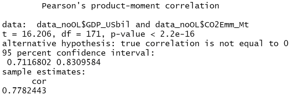
Figure 4. Correlation summary with no influential points
In evaluating the linear model, it was found that the correlation coefficient r = 0.78 with a p-value of p<2.2e-16, as seen in Figure 4. Because the p<0.05, the correlation coefficient is statistically significant; there is evidence for a positive linear relationship between GDP and CO2 emissions.
Conclusion
From this research we learned that the slope β1and correlation coefficient r are significant, there is a possibility of a linear relationship, but the diagnostic plots indicate that the assumptions of a linear regression model are not being met, specifically the assumptions of variation around the observation line and normal distribution of residuals are not being met. This suggests further work needs to be done in order to determine if there is a linear relationship between the two variables.
Possible limitations in this method include being unable to identify which countries have the highest GDP and CO2 emissions and being unable to identify which industries cause the most CO2 emissions. Possibilities for research of this topic includes investigating the relationship between GDP and CO2 emissions using alternative models and investigating regional trends of CO2 emissions and GDP
References
FocusEconomics. (2014, March 29). What is GDP? FocusEconomics | Economic Forecasts from the World's Leading Economists. Retrieved September 22, 2021, from https://www.focus-economics.com/economic-indicator/gdp.
“IEA Energy Atlas.” IEA Energy Atlas, energyatlas.iea.org/#!/tellmap/1378539487/3.
Taub, D. R. (2010). Effects of Rising Atmospheric Concentrations of Carbon Dioxide on Plants. Nature
news. Retrieved December 5, 2021, from
https://www.nature.com/scitable/knowledge/library/effects-of-rising-atmOspheric-conce
ntrations-of-carbon-13254108/.
World Bank. "CO2 Emissions (kt)." World Development Indicators. The World Bank Group, 2018, Retrieved September 22, 2021, from https://databank.worldbank.org/CEE-202-Project/id/e4cb3c21
World Bank. "GDP (current US$)." World Development Indicators. The World Bank Group, 2018, Retrieved September 22, 2021, from https://databank.worldbank.org/CEE-202-Project/id/e4cb3c21
Contributions
This deliverable is the result of cooperation of the following team members:
Syed Aisha contributed to cleaning data, writing R code, and contributing to the Results and Discussion section, Conclusion, and Abstract of the report.
Kelch Riley contributed to reformatting of the Introduction section, explanation in the Data and Methods section, and analysis of figures provided in the Results and Discussion section.
Wagner Alan contributed to writing and reworking the Introduction, analyzing figures in the Results and Discussion section, and editing the essay as a whole.
Luo Hongjie contributed to writing and interpreting the graph, discussing the figures, editing parts of the essay
Shao Emily contributed to writing the results and discussion section and proofreading all sections of the report.


Comments